Curve & Surface Fitting
geomdl includes 2 fitting methods for curves and surfaces: approximation and interpolation. Please refer to the
Curve and Surface Fitting page for more details on the curve and surface fitting API.
The following sections explain 2-dimensional curve fitting using the included fitting methods. geomdl also supports
3-dimensional curve and surface fitting (not shown here). Please refer to the Examples Repository for more examples on
curve and surface fitting.
Interpolation
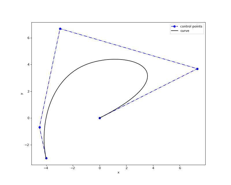
The following code snippet and the figure illustrate interpolation for a 2-dimensional curve:
 1from geomdl import fitting
 2from geomdl.visualization import VisMPL as vis
 3
 4# The NURBS Book Ex9.1
 5points = ((0, 0), (3, 4), (-1, 4), (-4, 0), (-4, -3))
 6degree = 3  # cubic curve
 7
 8# Do global curve interpolation
 9curve = fitting.interpolate_curve(points, degree)
10
11# Plot the interpolated curve
12curve.delta = 0.01
13curve.vis = vis.VisCurve2D()
14curve.render()
(Source code, png, hires.png, pdf)
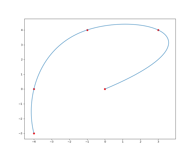
The following figure displays the input data (sample) points in red and the evaluated curve after interpolation in blue:
(Source code, png, hires.png, pdf)
Approximation
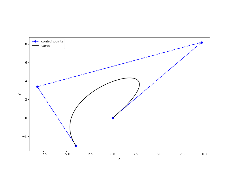
The following code snippet and the figure illustrate approximation method for a 2-dimensional curve:
 1from geomdl import fitting
 2from geomdl.visualization import VisMPL as vis
 3
 4# The NURBS Book Ex9.1
 5points = ((0, 0), (3, 4), (-1, 4), (-4, 0), (-4, -3))
 6degree = 3  # cubic curve
 7
 8# Do global curve approximation
 9curve = fitting.approximate_curve(points, degree)
10
11# Plot the interpolated curve
12curve.delta = 0.01
13curve.vis = vis.VisCurve2D()
14curve.render()
(Source code, png, hires.png, pdf)
The following figure displays the input data (sample) points in red and the evaluated curve after approximation in blue:
(Source code, png, hires.png, pdf)
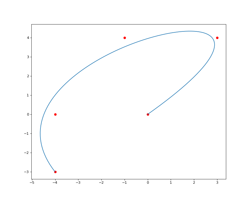
Please note that a spline geometry with a constant set of evaluated points may be represented with an infinite set of control points. The number and positions of the control points depend on the application and the method used to generate the control points.